← Octo-TIGER / All test problemsSteady diffusion

Equilibrium sphere

A smooth spherical emitter balances outward radiation transport. An error-function solution describes its steady diffusion equilibrium.

Simulation movies

Equilibrium Sphere · max level 2 · EULER

equilibrium sphere | EULER | level 2 | AMR

Central z=0+ radiation energy slice with faint cell mesh and equal-length flux direction arrows. Fixed color limits; actual stored Silo times held without solution interpolation. The maps show the full simulation domain without cropping. Equilibrium-maintenance test; a nearly stationary field is expected.

Download MP4 · Rendering details · Simulation report

All campaign movies

The experiment

Physical setup

A Gaussian light source is centered in a stationary medium of prescribed opacity χ. It emits total luminosity ℒ over all space, with a smooth width w:

q(r) = ℒ exp(−r²/w²) / (π3/2 w³),   r = |x|

The domain starts from the steady diffusion solution on top of background Ebg. Boundaries are nonperiodic: ghost cells are fixed to cell averages of that same analytic equilibrium. The incoming background is part of this boundary state. The gas remains fixed; the source adds radiation energy and the medium damps flux.

The standard CGS templates use w = 6 × 10⁹ cm, χ = 1.6666666667 × 10⁻¹⁰ cm−1, Ebg = 1 erg/cm³, and ℒ = 2.698132122 × 10²⁹ erg/s. This is a smooth Gaussian emitter. The saved settings below give the actual values used.

The standard runner uses a uniform cubic grid with hydrodynamics and gravity disabled. Its CGS box spans −3 × 10¹⁰ to +3 × 10¹⁰ cm on each axis, with c = 2.99792458 × 10¹⁰ cm/s and default final time 4 s. Opt-in adaptive runs are identified below; N = INX × 2level then describes their configured finest equivalent resolution. Each completed run below lists its recorded parameters.

The comparison

Comparison and interpretation

In steady isotropic diffusion, D = c/(3χ), ∇ · F = q, and F = −D∇E. Integrating the enclosed Gaussian luminosity gives

E(r) = Ebg + [3χℒ/(4πc)] erf(r/w)/r
F(x) = [ℒ/(4πr³)] [erf(s) − 2s e−s²/√π] x,   s = r/w

The apparent singularities are removable: E(0) = Ebg + 3χℒ/(2π3/2cw) and F(0) = 0. The implementation uses series expansions near the origin.

Initial, boundary, and comparison states are cell averages evaluated with four-point Gauss–Legendre quadrature on each axis (64 samples per cell). The smooth-field averages therefore have quadrature error. The Gaussian source has an exact cell integral, evaluated as a product of three error-function differences:

q̄ = (ℒ/Δx³) ∏d=x,y,z ½ {erf[(xd + Δx/2)/w] − erf[(xd − Δx/2)/w]}

The prescribed source adds Δt q̄ to energy and damps flux at rate cχ. Its numerical integration depends on the recorded method, as described below. The steady reference itself is independent of time.

What this test measures

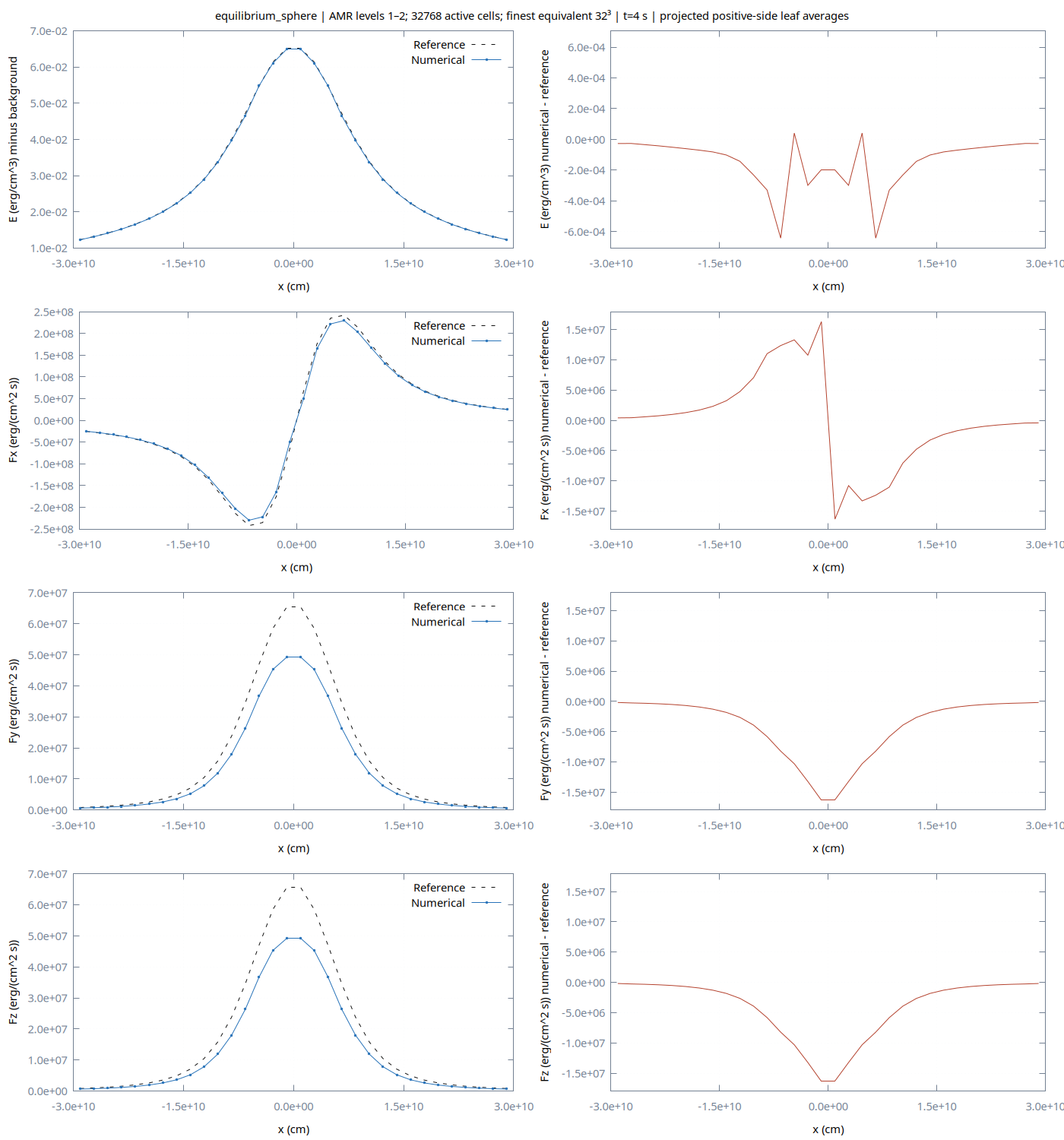
This is a diffusion-limit equilibrium test. Nonlinear M1 has an anisotropic pressure at finite flux, so the diffusion solution need not remain exactly stationary in that model. Errors can reflect closure differences, transport/source splitting, discretization, and quadrature. The plots measure equilibrium drift and Cartesian directional effects as resolution changes.

Energy injected inside the finite cube should balance its outward transport and the change in stored energy. ℒ is the all-space luminosity; use the measured in-domain source budget rather than assuming the finite cube receives exactly ℒ. Symmetry can make net flux integrals very small, which is why their conservation normalization includes an energy-based scale.

Measured results

All resolutions

LevelGridBatch status
232³Ready

Convergence requires at least two completed, comparable resolutions.

Full-volume norms and orders

GridFieldNormErrorOrderError units
AMR levels 1–2; 32768 active cells; finest equivalent 32³erL12.019307e-05—erg/cm³
AMR levels 1–2; 32768 active cells; finest equivalent 32³erL25.151584e-05—erg/cm³
AMR levels 1–2; 32768 active cells; finest equivalent 32³erLinf6.424667e-04—erg/cm³
AMR levels 1–2; 32768 active cells; finest equivalent 32³fxL12.596979e+05—erg/(cm² s)
AMR levels 1–2; 32768 active cells; finest equivalent 32³fxL29.097040e+05—erg/(cm² s)
AMR levels 1–2; 32768 active cells; finest equivalent 32³fxLinf1.630999e+07—erg/(cm² s)
AMR levels 1–2; 32768 active cells; finest equivalent 32³fyL12.596979e+05—erg/(cm² s)
AMR levels 1–2; 32768 active cells; finest equivalent 32³fyL29.097040e+05—erg/(cm² s)
AMR levels 1–2; 32768 active cells; finest equivalent 32³fyLinf1.630999e+07—erg/(cm² s)
AMR levels 1–2; 32768 active cells; finest equivalent 32³fzL12.596979e+05—erg/(cm² s)
AMR levels 1–2; 32768 active cells; finest equivalent 32³fzL29.097040e+05—erg/(cm² s)
AMR levels 1–2; 32768 active cells; finest equivalent 32³fzLinf1.630999e+07—erg/(cm² s)

AMR levels 1–2; 32768 active cells; finest equivalent 32³ / level 2

Recorded setup and run provenance
OriginOcto-TIGER application
DomainCube of side 6.000000e+10 cm; centered at the origin
ResolutionAMR levels 1–2; 32768 active cells; finest equivalent 32³; finest Δx = 1.875000e+09 cm
Slice geometryAMR: positive-side cells touching z=0, projected as constant leaf averages. Centers have z=leaf_dx/2; the ray similarly touches y=0. This is not a common cell-center plane. Raw CSV preserves native cells; display CSV repeats coarse values on finest pixels, retaining source dx/z. Full-volume norms use actual leaf volumes; uniform-grid convergence orders are not reported.
Final comparison time4.000000e+00 s
Radiation integrationLegacy first-order radiation update
Radiation backendcpu
Physical light speed2.997925e+10 cm/s
Reduced-speed factor α1.000000e+00
Radiation transport speed2.997925e+10 cm/s
Periodic boundariesoff
Hydrodynamicsoff
Gravityoff
Implicit radiation sourceon
Uniform gridoff
CFL0.4
Timestep cap0.040000000000000001 s
Output interval0.20000000000000001 s
Background energy density1 erg/cm³
Scattering coefficient χ1.6666666666666666e-10 cm⁻¹
Gaussian width w6000000000 cm
All-space luminosity ℒ2.6981321220000001e+29 erg/s
{
  "adaptive": true,
  "background": 1.0,
  "c": 29979245800.0,
  "case": "equilibrium_sphere",
  "cells": 32,
  "command": [
    "/home/dmarce1/workspace/octotiger/radiation_results/results/local-euler-ader2-20261011-restart-01/.campaign/launch-solver",
    "/home/dmarce1/workspace/octotiger/radiation_results/results/local-euler-ader2-20261011-restart-01/.campaign/runtime/octotiger",
    "--config_file=/home/dmarce1/workspace/octotiger/radiation_results/results/local-euler-ader2-20261011-restart-01/runs/l2/equilibrium_sphere/euler/equilibrium_sphere/l2/run.ini",
    "--hpx:threads=12"
  ],
  "comparison_signature": {
    "atomic_mass": "1",
    "atomic_number": "1",
    "cfl": "0.4",
    "code_to_cm": "1",
    "code_to_g": "1",
    "code_to_s": "1",
    "disable_analytic": "off",
    "disable_diagnostics": "on",
    "gravity": "off",
    "hard_dt": "0.040000000000000001",
    "hydro": "off",
    "hydro_device_kernel_type": "OFF",
    "hydro_host_kernel_type": "LEGACY",
    "monopole_device_kernel_type": "OFF",
    "multipole_device_kernel_type": "OFF",
    "n_species": "1",
    "omega": "0",
    "periodic": "off",
    "problem": "RADIATION_EQUILIBRIUM_SPHERE",
    "rad_implicit": "on",
    "rad_test_amplitude": "0.01",
    "rad_test_background": "1",
    "rad_test_chi": "1.6666666666666666e-10",
    "rad_test_luminosity": "2.6981321220000001e+29",
    "rad_test_width": "6000000000",
    "radiation": "on",
    "radiation_integrator": "euler",
    "radiation_reduced_c_factor": "1",
    "stop_step": "100000",
    "stop_time": "4",
    "study_config_sha256": "a7ffc569ea95d062e7f4d4b96786783a2c678d14b32981f7e48f1a25899973e6",
    "unigrid": "off",
    "xscale": "30000000000"
  },
  "config": {
    "atomic_mass": "1",
    "atomic_number": "1",
    "cfl": "0.4",
    "code_to_cm": "1",
    "code_to_g": "1",
    "code_to_s": "1",
    "datadir": "/home/dmarce1/workspace/octotiger/radiation_results/results/local-euler-ader2-20261011-restart-01/runs/l2/equilibrium_sphere/euler/equilibrium_sphere/l2/",
    "disable_analytic": "off",
    "disable_diagnostics": "on",
    "disable_output": "off",
    "gradient_refine_buffer": "0",
    "gradient_refine_coarsen_factor": "0.80000000000000004",
    "gradient_refine_field": "radiation_energy",
    "gradient_refine_floor": "1.0000000000000001e-30",
    "gradient_refine_mode": "absolute",
    "gradient_refine_threshold": "1.7104563249411638e-12",
    "gravity": "off",
    "hard_dt": "0.040000000000000001",
    "hydro": "off",
    "hydro_device_kernel_type": "OFF",
    "hydro_host_kernel_type": "LEGACY",
    "max_level": "2",
    "min_level": "1",
    "monopole_device_kernel_type": "OFF",
    "multipole_device_kernel_type": "OFF",
    "n_species": "1",
    "odt": "0.20000000000000001",
    "omega": "0",
    "periodic": "off",
    "problem": "RADIATION_EQUILIBRIUM_SPHERE",
    "rad_implicit": "on",
    "rad_test_amplitude": "0.01",
    "rad_test_background": "1",
    "rad_test_chi": "1.6666666666666666e-10",
    "rad_test_luminosity": "2.6981321220000001e+29",
    "rad_test_width": "6000000000",
    "radiation": "on",
    "radiation_backend": "cpu",
    "radiation_integrator": "euler",
    "radiation_reduced_c_factor": "1",
    "stop_step": "100000",
    "stop_time": "4",
    "unigrid": "off",
    "xscale": "30000000000"
  },
  "conservation": [
    {
      "boundary": 1.0796930626199439e+30,
      "boundary_fraction": 0.0049294798111907635,
      "field": "er",
      "final": 2.1902734851326454e+32,
      "final_fraction": 0.9999979901462385,
      "initial": 2.1902778872708958e+32,
      "initial_fraction": 1.0,
      "integral_units": "erg",
      "max_abs_residual": 2.5051272927248384e+16,
      "max_normalized_error": 1.143748611664179e-16,
      "normalization_basis": "abs(initial_energy)",
      "normalization_scale": 2.1902778872708958e+32,
      "normalized_error": 6.682576158037901e-17,
      "normalized_residual": -6.682576158037901e-17,
      "raw_change": -4.402138250420552e+26,
      "residual": -1.4636698788954112e+16,
      "source": 1.0792528487949165e+30,
      "source_fraction": 0.004927469957429349,
      "zero_initial_flux_relative_tolerance": 1.4210854715202004e-14
    },
    {
      "boundary": 5.01220172575577e+24,
      "boundary_fraction": 7.633234774997108e-19,
      "field": "fx",
      "final": -8.49841499475799e+23,
      "final_fraction": -1.2942495218618124e-19,
      "initial": 2.767011611056433e+21,
      "initial_fraction": 4.213966318195612e-22,
      "integral_units": "erg cm/s",
      "max_abs_residual": 1.9857919995348332e+22,
      "max_normalized_error": 3.024223161025051e-21,
      "normalization_basis": "c * abs(initial_energy)",
      "normalization_scale": 6.566287915279887e+42,
      "normalized_error": 2.9290577550058e-21,
      "normalized_residual": -2.9290577550058e-21,
      "raw_change": -8.526085110868555e+23,
      "residual": -1.923303653985142e+22,
      "source": 4.1788262512087656e+24,
      "source_fraction": 6.364061864367157e-19,
      "zero_initial_flux_relative_tolerance": 1.4210854715202004e-14
    },
    {
      "boundary": -4.0828400019270235e+25,
      "boundary_fraction": -6.217881479772111e-18,
      "field": "fy",
      "final": 1.642018476977182e+24,
      "final_fraction": 2.500679985652428e-19,
      "initial": 5.165088340638674e+21,
      "initial_fraction": 7.866070460631809e-22,
      "integral_units": "erg cm/s",
      "max_abs_residual": 4.4092330022184256e+23,
      "max_normalized_error": 6.714955328044707e-20,
      "normalization_basis": "c * abs(initial_energy)",
      "normalization_scale": 6.566287915279887e+42,
      "normalized_error": 6.401787397830804e-20,
      "normalized_residual": 6.401787397830804e-20,
      "raw_change": 1.6368533886365434e+24,
      "residual": 4.2035979226567483e+23,
      "source": -3.961190642289937e+25,
      "source_fraction": -6.032617962231239e-18,
      "zero_initial_flux_relative_tolerance": 1.4210854715202004e-14
    },
    {
      "boundary": -8.493766415251416e+24,
      "boundary_fraction": -1.2935415755203554e-18,
      "field": "fz",
      "final": 2.5759033424528018e+23,
      "final_fraction": 3.9229217111522353e-20,
      "initial": -3.947603231773844e+21,
      "initial_fraction": -6.01192528062574e-22,
      "integral_units": "erg cm/s",
      "max_abs_residual": 2.658268054741915e+23,
      "max_normalized_error": 4.048357441890525e-20,
      "normalization_basis": "c * abs(initial_energy)",
      "normalization_scale": 6.566287915279887e+42,
      "normalized_error": 3.943254098637529e-20,
      "normalized_residual": 3.943254098637529e-20,
      "raw_change": 2.6153793747705402e+23,
      "residual": 2.589254173476149e+23,
      "source": -8.491153895121977e+24,
      "source_fraction": -1.2931437068671458e-18,
      "zero_initial_flux_relative_tolerance": 1.4210854715202004e-14
    }
  ],
  "dx": 1875000000.0,
  "executable_sha256": "fc0e982bc397d82e25c7105cff6a97a514f09c57439e579587f4ddf6f6a8fa14",
  "inx": 8,
  "length": 60000000000.0,
  "level": 2,
  "max_level": 2,
  "mesh": {
    "full_mesh": {
      "last_regrid_step": 770.0,
      "last_regrid_time": 4.0,
      "leaf_blocks": 64,
      "leaf_cells": 32768,
      "levels": {
        "2": {
          "leaf_blocks": 64,
          "leaf_cells": 32768
        }
      }
    },
    "geometry": "Positive-side leaf cells touching geometric z=0; cell centers have z=leaf_dx/2",
    "native_slice_cells": 1024,
    "projection": "Piecewise-constant leaf cell averages onto finest display pixels; raw CSV retains native cells",
    "slice_cells_by_level": {
      "2": 1024
    }
  },
  "mesh_description": "Adaptive Cartesian leaves; cells/dx denote configured finest equivalent resolution",
  "min_level": 1,
  "movie_capture": {
    "hard_dt": 0.04,
    "odt": 0.2,
    "requested_snapshots": 21,
    "steps_per_output_check": 5
  },
  "norms": {
    "er": {
      "L1": 2.019307e-05,
      "L2": 5.151584e-05,
      "Linf": 0.0006424667
    },
    "fx": {
      "L1": 259697.9,
      "L2": 909704.0,
      "Linf": 16309990.0
    },
    "fy": {
      "L1": 259697.9,
      "L2": 909704.0,
      "Linf": 16309990.0
    },
    "fz": {
      "L1": 259697.9,
      "L2": 909704.0,
      "Linf": 16309990.0
    }
  },
  "origin": "Octo-TIGER application",
  "physical_c": 29979245800.0,
  "radiation_ader_version": 0,
  "radiation_backend": "cpu",
  "radiation_equations": "physical-c",
  "radiation_integrator": "euler",
  "radiation_reduced_c_factor": 1.0,
  "status": "complete",
  "study_config_sha256": "a7ffc569ea95d062e7f4d4b96786783a2c678d14b32981f7e48f1a25899973e6",
  "time": 4.0,
  "transport_c": 29979245800.0,
  "units": {
    "chi": "1/cm",
    "energy_density": "erg/cm^3",
    "flux": "erg/(cm^2 s)",
    "length": "cm",
    "luminosity": "erg/s",
    "mass": "g",
    "source": "erg/(cm^3 s)",
    "system": "CGS",
    "time": "s"
  }
}

Final fields and profiles

AMR: positive-side cells touching z=0, projected as constant leaf averages. Centers have z=leaf_dx/2; the ray similarly touches y=0. This is not a common cell-center plane. Raw CSV preserves native cells; display CSV repeats coarse values on finest pixels, retaining source dx/z. Full-volume norms use actual leaf volumes; uniform-grid convergence orders are not reported.

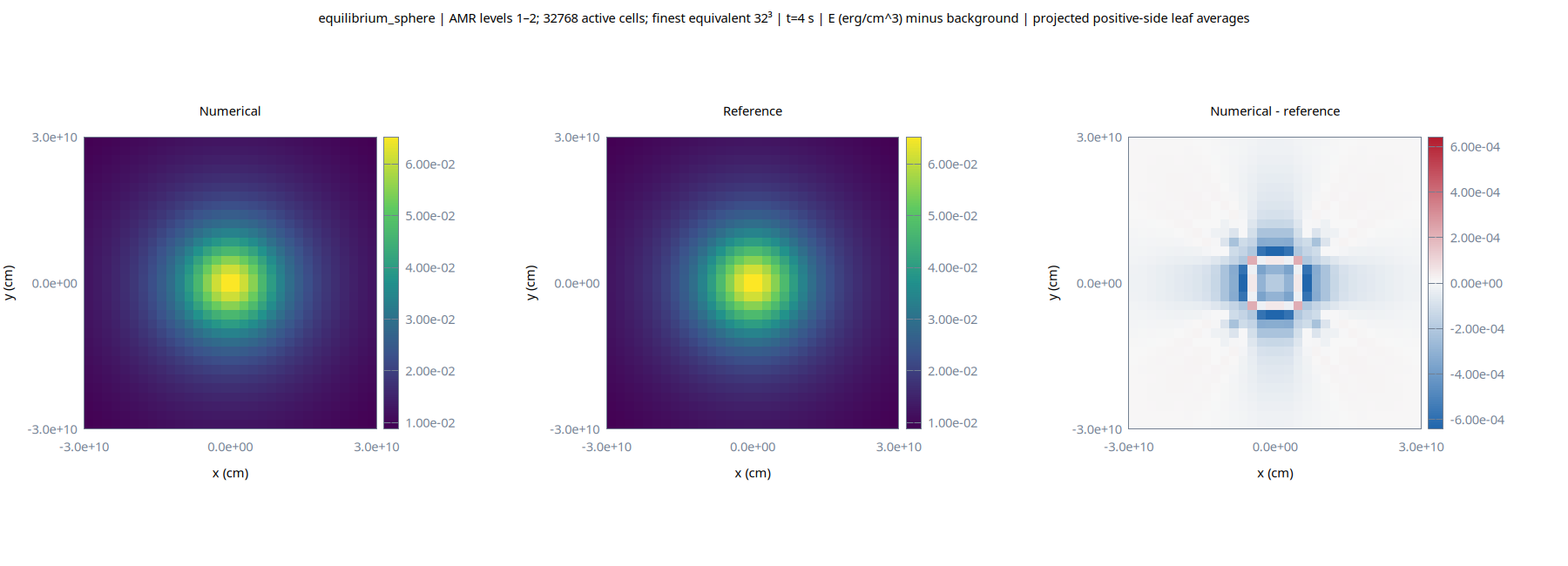
Numerical, reference, and signed-error energy slices. AMR: positive-side cells touching z=0, projected as constant leaf averages. Centers have z=leaf_dx/2; the ray similarly touches y=0. This is not a common cell-center plane. Raw CSV preserves native cells; display CSV repeats coarse values on finest pixels, retaining source dx/z. Full-volume norms use actual leaf volumes; uniform-grid convergence orders are not reported.
Numerical, reference, and signed-error energy slices. AMR: positive-side cells touching z=0, projected as constant leaf averages. Centers have z=leaf_dx/2; the ray similarly touches y=0. This is not a common cell-center plane. Raw CSV preserves native cells; display CSV repeats coarse values on finest pixels, retaining source dx/z. Full-volume norms use actual leaf volumes; uniform-grid convergence orders are not reported. · PDF
Numerical/reference line profiles and signed errors for all four radiation fields
Numerical/reference line profiles and signed errors for all four radiation fields · PDF
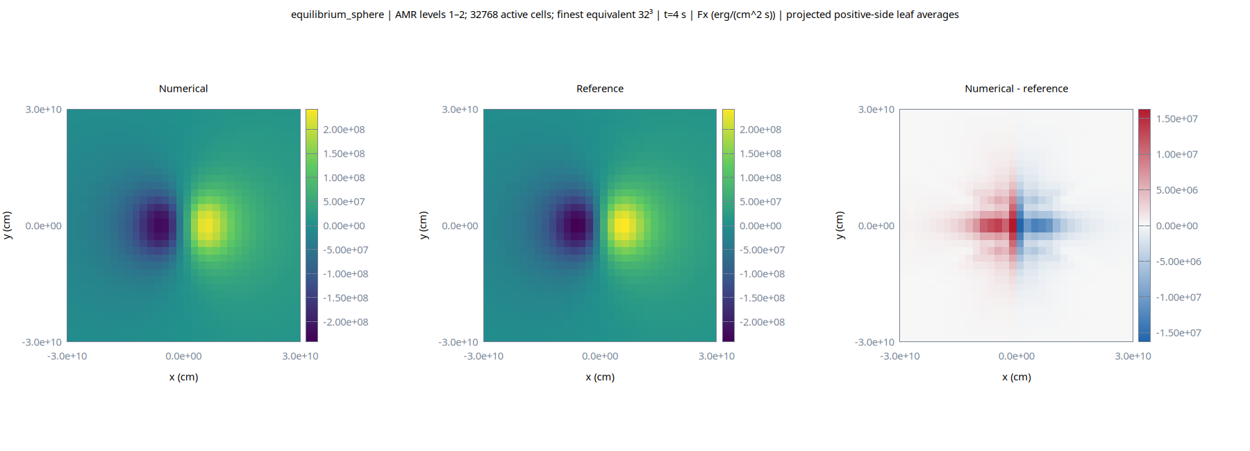
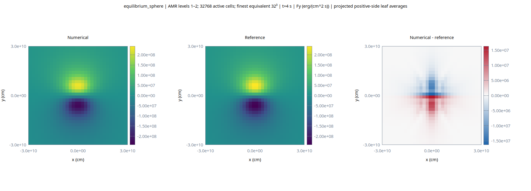
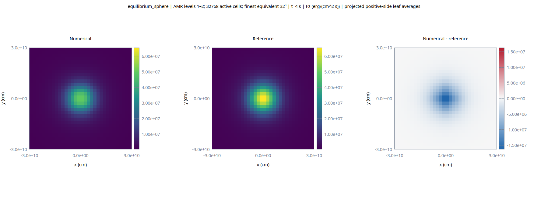
All three flux maps
fx: numerical, reference, and signed-error slice
fx: numerical, reference, and signed-error slice · PDF
fy: numerical, reference, and signed-error slice
fy: numerical, reference, and signed-error slice · PDF
fz: numerical, reference, and signed-error slice
fz: numerical, reference, and signed-error slice · PDF

Movies

No completed movie is available for this resolution.

Conservation

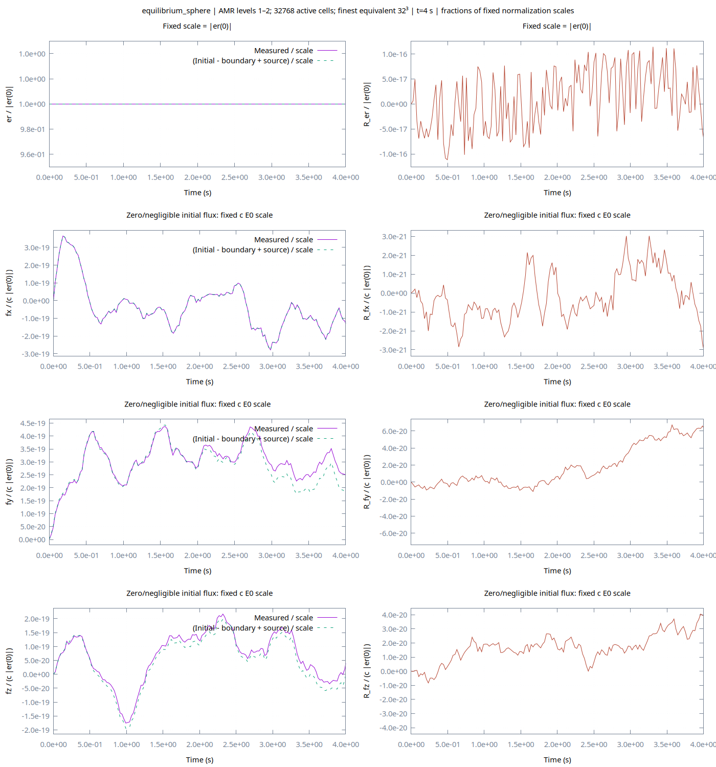
All values below are dimensionless fractions of the fixed normalization scale.
FieldScaleQ(0)/scaleQ(t)/scaleBoundary B/scaleSource S/scaleResidual R/scaleMaximum |R|/scale
er|Q(0)|1.000000e+009.999980e-014.929480e-034.927470e-03-6.682576e-171.143749e-16
fxc |E₀| (zero/negligible initial flux)4.213966e-22-1.294250e-197.633235e-196.364062e-19-2.929058e-213.024223e-21
fyc |E₀| (zero/negligible initial flux)7.866070e-222.500680e-19-6.217881e-18-6.032618e-186.401787e-206.714955e-20
fzc |E₀| (zero/negligible initial flux)-6.011925e-223.922922e-20-1.293542e-18-1.293144e-183.943254e-204.048357e-20
Integrated radiation budgets and their transport/source-corrected residuals
Integrated radiation budgets and their transport/source-corrected residuals · PDF

Data and reproducibility

Reading the results

Errors, budgets, and movies

Every norm uses the full three-dimensional domain, with cell-volume weighting. Here e = numerical − reference and V is the domain volume:

L1 = Σ |e| ΔV / V,   L2 = √(Σ e² ΔV / V),   L∞ = max |e|
p = ln(errorcoarse / errorfine) / ln(Δxcoarse / Δxfine)

Orders require two completed runs with matching physical time, configuration, units, executable, and origin. An exact zero error has no logarithmic order. The central slice and line profiles are visual diagnostics: the report slice is the cell layer at z = Δx/2, and its line profile is at y = z = Δx/2.

Conservation is assessed using the measured domain integrals and the signed cumulative boundary and source budgets:

R(t) = Q(t) − Q(0) + B(t) − S(t)

B is outward transport and S is the source change. Conservation plots and this page's budget tables show fractions of the initial totals: Q(t)/D, [Q(0) − B(t) + S(t)]/D, and the signed residual R(t)/D. The denominator D = |Q(0)| is fixed for the entire history. It never grows with the current total or accumulated transport/source budgets. A negative initial flux therefore starts at −1, and the plotted fraction retains its sign.

A component whose initial net flux is zero or negligible cannot be divided by its own initial total. It instead uses the fixed scale D = c |E₀|, where E₀ is the initial integrated radiation energy. This fallback is labeled on its panels and in the table. “Negligible” means |Q(0)|/(c |E₀|) ≤ 64ε ≈ 1.421085 × 10⁻¹⁴, with ε the double-precision machine epsilon. This prevents roundoff left by cancellation in a symmetric field from becoming the denominator. For the initially cold Marshak case, the prescribed bath sets D = Ebath V for energy and D = c Ebath V for flux, with Ebath = 4/c. These scales remain fixed even though radiation enters the initially empty domain.

Raw histories and dimensional summary columns remain in physical units: energy integrals in erg, physical-flux integrals in erg cm/s for CGS runs. Dividing a flux integral by c² gives radiation momentum. Fraction-history CSV files are dimensionless except for their time column; summary files record each denominator and its basis. Maximum fractional residuals use the same fixed denominator as the final residual.

For runs labeled RSLA, these budgets check the modified radiation equations. They do not establish conservation of physical gas-plus-radiation energy. With reduced-speed factor α, the closed-system coupled invariants are Egas + Er/α and gas momentum + F/(αc²), with physical c in the closure. Compare multiple α values before interpreting an RSLA result as an approximation to physical-c evolution.

Movies show the numerical Silo states with a fixed color range for each movie. Recorded states are held for their actual simulation-time gaps; intermediate solutions are not interpolated. The 3D option shows the domain's exterior surface. Movies and plots retain their recorded physical units.

Sources & provenance

Where this problem comes from

This smooth Gaussian-emitter test is defined by equilibriumSphere, sphereAverage, and bulbSourceAverage in octotiger/test_problems/radiation/profiles.hpp. Its reference follows by solving the steady diffusion equation for that source. The available implementation does not identify it as a verbatim published sphere benchmark, so the provenance here is the suite's analytic construction.

Radiation method context

Skinner & Ostriker (2013), “A Two-moment Radiation Hydrodynamics Module in Athena Using a Time-explicit Godunov Method,” ApJS 206, 21, provides context for the two-moment M1 system and source integration. For the radiation-only Gaussian and sphere cases, Euler uses backward-Euler damping: Fn+1 = F*/(1 + cχΔt), where F* is the flux after transport. This uses the algebra of their equations (42b)–(43) with θ = 1 and prescribed χ. Their paper neglects scattering; the suite reuses that damping formula for its prescribed scattering medium. ADER2 revision 6 uses the same two-stage Radau IIA local integration for all eight problems. Transport is evaluated on the old state, a predicted time average and a corrected time average, with reconstruction recomputed each time. Prescribed-medium constraints are applied within the implicit stages: the Gaussian and sphere tests hold the material fixed; Marshak holds density and velocity fixed while thermal energy evolves; streaming disables interaction. The coupled problems evolve gas and radiation together on one shared timestep. This implementation does not yet include gravity, and uniform stiff coupled second-order accuracy remains unresolved. Historical revision 5 used exponential affine-forcing solutions for prescribed scattering, SDIRK2 for stationary Marshak heating, and Radau stages for coupled hydro–radiation. Those saved results retain their original method revision and do not validate revision 6. Here the formulas use physical light speed; reduced-speed runs retain their recorded transport speed.

The solver's M1 implementation also cites Hanawa & Audit (2014), “Reformulation of the M1 model of radiative transfer,” JQSRT 145, 9–16. These references describe the numerical/physical framework; the exact test definitions are the source functions identified above.

Reproducing this batch

Descriptions document the reviewed source implementation. Older or edited solver versions can use different profile constants or averaging rules; these are not all encoded in run.ini. Use the run metadata, executable hash, and saved batch source hashes to identify the implementation behind a result. A source path or descriptive formula alone is not proof of the executable's contents.